Multivariable Calculus
Partial Differentiation
Explicit Differentiation
Basic Example
The rule of thumb is to treat whatever variable we are not taking the derivative of as a constant:
f(x,y) = x^3 y+2x^2+9y^2+xy+10
We may wish to find the derivative of f with respect to x:
df/dx =
In this case we need to treat y as a constant. The best way to think of this is that dz/dx is the path that would be available if we were to walk in any direction keeping our y-coordinate fixed.
df/dx = 3x^2y + 4x + 0 + y + 0
df/dx = 3x^2y + 4x + y
To break this down a little, whenever we had an x multiplied by y we were not able to just get rid of the y as its treated as a constant. However, an isolated y or constant we just treat as 0.
Chain Rule Example
f(x,y) = (x+y^2)^3
In this case we apply the chain rule:
{insert chain rule here}
df/dx = 3(x + y^2)^2 * (1+0)
df/dx = 3(x + y^2)^2
Trigonometric Example
f(x,y) = x^2 y + sin(y)
df/dx = 2xy + 0
df/dx = 2xy
df/dy = x^2 + cos(y)
Implicit Differentiation
Implicit differentiation includes some type of equality, as below:
z(x,y) = xyz = x – y + z
The trick to it is that we need to differentiate with respect to x, so we apply the typical derivative rule, but whenever we see the z term we need to multiply it by dz/dx as follows:
z(x,y) = xyz = x – y + z
dz/dx = yz*dz/dx = 1 + z*dz/dx
Why have we done this? the y on the right hand side disappears because it is treated as a constant, the y on the left remains because it is multiplied by x.
Let’s try an example:
z(x,y)= x^2+y^2+z^2=10
dz/dx =
−x/z,
Gradient
The gradient points in the direction of steepest ascent.
The length of the gradient vector measures how steep the ascent is.
Critical Points of a Function
Critical points occur when the partial derivative with respect to one of the variables equals 0. Example:
To find an evaluate critical points of the function:
x^3 – 15x^2 – 20y^2 + 5
Step 1: Take the first-order and second-order partial derivatives with respect to each variable.
fx (x, y) = 3x^2-30x
fy (x, y) = -40y
fxx (x, y) =
fyy (x, y) =
fxy (x, y) =
Step 2: Find critical points by solving the system of equations:
Critical points occur when the first derivatives equal 0:
3x^2-30x = 0
-40y = 0
Step 3: Find the discriminant of f(x,y) at critical point (a,b)
D(a,b) = fxx(a,b)*fyy(a,b) – [fxy(a,b)]^2
Step 4: Classifying critical points using second order partial derivative test:
General Solutions to Differential Equations
Initial Value Problems
Fourier Series
We use the Fourier series when we have a periodic function:
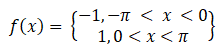
The above simply means that when x is between negative pi and 0, y= -1 and when x is between 0 and pi, y = 1. The function changes sign at the origin, basically.
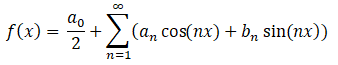
Let’s break down how the series works in practice:
a0 is the average level of the function, most often it is 0 for the origin but not always.
an is the
bn is the
The rule is: if the function is odd (meaning it alternates between negative and positive), only sins. if the function is even (meaning the values are all positive or all negative), only cosines.
Fourier Series Examples
Even Function
Step 1: Write the Fourier Equation in Full
Step 2: Determine whether it is an odd or even function
Step 3: Finding an
Odd Function
Step 1: Write the Fourier Equation in Full
Step 2: Determine whether it is an odd or even function
The function is an odd function so we know that a0 and an will be 0, so remove those elements from consideration and find only bn.
Step 3: Finding bn
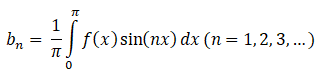
The above formula is designed for odd and even functions, but we can take a shortcut:
The 2 will be negative because the integral of sine is negative cosine:
Cos(0) is equal to 1, so the answer will be:
Taylor Series
Taylor Series Examples
f(x) = (sin x)^3
Step 1: Write the Taylor Series Equation

Step 2: Find associated coefficients
Euler’s Method
Euler’s Method Examples
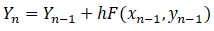
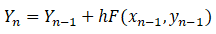
Step 1: Write Euler’s Method Formula
Step 2: Set out the question, defining it.
Δx = 1
1 ≤ x ≤ 4
y(1) = 1
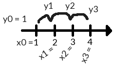
As the above figure shows, we take steps from 1 onwards, in steps of 1, to get to 4.
Step 3: Calculate y values
Our first y value is given by the initial condition:
y0 = 1
y1 = y0 + x0(1+y0) = 1 + 1(1+1) = 3
y2 = y1 + x1(1+y1) = 3 + 2(1+3) = 11
y3 = y2 + x2(1+y2) = 11 + 3(1+11) = 47
Ans:
y(4) = 47
Identity Matrix
1*x = x
The 1 is the identity. When we apply this concept to matrix multiplication, becuase matrix multiplication is ordered row * column, we get the following:
IM = M
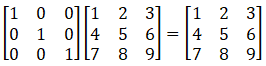
The identity matrix is thus:

How this works is that the first item in the matrix ‘M’, 1, is equal to one after being multiplied by the identity matrix because 1*1 + 0*4 + 0*7 = 1.
Eigenvalues of a Matrix
Calculating Eigenvalues of a Matrix Examples
Eigenvectors of a Matrix
Calculating Eigenvectors of a Matrix
Reference
http://www.columbia.edu/itc/sipa/math/calc_rules_multivar.html
http://personal.maths.surrey.ac.uk/S.Zelik/teach/calculus/partial_derivatives.pdf
https://www.youtube.com/watch?v=mU9xb-j7cOI